import torch
import torch.nn as nnAttention Mechanisms (chapter 3)
This notebook explores attention mechanisms (including self-attention) based on Sebastian Raschka’s book (Chapter 3), implementing basic self-attention, causal self-attention, and multi-headed self-attention (as shown in the figure below).
Acknowledgment
All concepts, architectures, and implementation approaches are credited to Sebastian Raschka’s work. This repository serves as my personal implementation and notes while working through the book’s content.
Resources

Simplified self-attention
This mechanism is inspired by the Bahdanau attention mechanism (named after the author of the paper that introduced this mechanism). When generating an output token, the decoder has access to all input tokens selectively. The importance of each input token is determined by an attention weight. More on the Bahdanau attention mechanism is shown in appendix B of the book.
Note that self-attention refers to the fact that we are computing attention / importance weights with respect to a single input sequence. In other words, self-attention asseses and learns the relationships and dependencies between various parts of the input iteself.

In the figure above, we are computing the context vector z(2) for the query vector x(2). That context vector z(2) is based on other input elements \(x^{(i)}\) in the input sequence \(x\) (of length T) where the importance of each input element is determined by attention weights \(\alpha_{ij}\).
Note that attention weights \(\alpha_{ij}\) are the normalized version of attention scores \(\omega_{ij}\) we’ll see later on.
A context vector can be thought of as an ‘enriched’ embedding vector that carries context from all other token embedding vectors in the input sequence.
A simple example (single query vector)
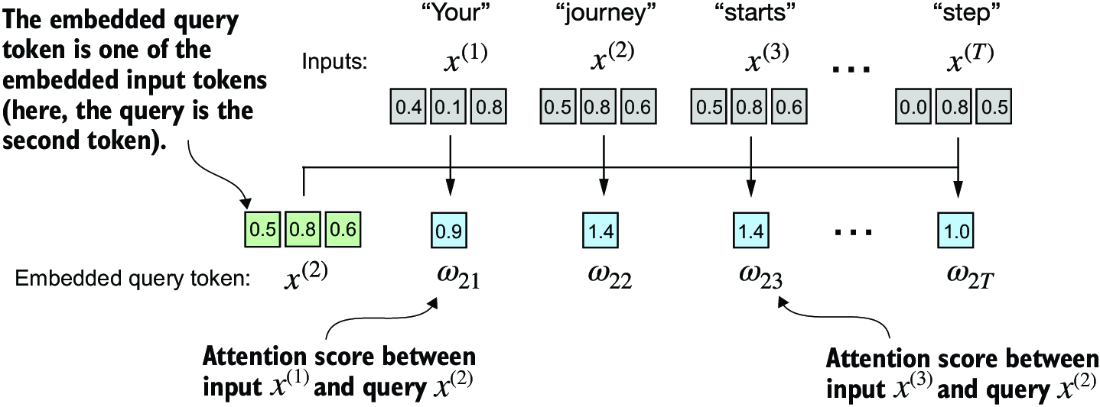
These attention scores \(\omega_{ij}\) are then normalized to arrive at attention weights \(\alpha_{ij}\). Normalization helps with interpretability and maintaining stability during the training process of LLMs.

Computing the context vector is simply the attention-weighted sum of all input elements.

# Define the input sequence (T = 6).
inputs = torch.tensor(
    [
        [0.43, 0.15, 0.89],  # Your    (x^1)
        [0.55, 0.87, 0.66],  # journey (x^2)
        [0.57, 0.85, 0.64],  # starts  (x^3)
        [0.22, 0.58, 0.33],  # with    (x^4)
        [0.77, 0.25, 0.10],  # one     (x^5)
        [0.05, 0.80, 0.55],  # step    (x^6)
    ]
)

# Compute the attention scores (for the second element of the sequence x^2)
# NOTE: The attention score computes similarity based on the dot product of the query and key vectors,
#       which measures how aligned the query and key vectors are (a higher dot product indicates a
#       greater degree of alignment, i.e. similarity between two vectors). A dot product is essentially
#       a concise way of multiplying two vectors element-wise and summing the result.
# NOTE: In the context of self-attention, the dot product determines the amount of attention the query
#       should "pay" to each key in the input sequence.

# 1. Via basic for-loops.
query = inputs[1]  # Python uses 0-based indexing.
attn_scores = torch.empty(inputs.shape[0])
for i, x_i in enumerate(inputs):
    attn_scores[i] = torch.dot(x_i, query)
print(attn_scores)


# 2. Via matrix multiplication.
attn_scores_mm = (
    query @ inputs.T
)  # The @ operator is syntactic sugar for matrix multiplication.
print(attn_scores_mm)

# Verify that the two methods yield the same attention scores.
assert torch.allclose(attn_scores, attn_scores_mm)

# Normalize the attention scores to get the attention weights.
# 1. Via a naive approach.
attn_weights = attn_scores / torch.sum(attn_scores)
print(f"Attention weights: {attn_weights} (sum: {torch.sum(attn_weights)})")

# 2. Via the softmax function.
# NOTE: Softmax handles extreme values more gracefully and offers more favorable gradient properties
#       during training.
# NOTE: Since the softmax function ensures that attention weights are always positive and sum to 1,
#       we can interpret the attention weights as probabilities.
attn_weights_softmax = torch.nn.functional.softmax(attn_scores, dim=0)
print(
    f"Attention weights: {attn_weights_softmax} (sum: {torch.sum(attn_weights_softmax)})"
)

# Compute the context vector z(2) for the query vector x(2).
# 1. Via a naive approach via a for-loop.
context_vector_2 = torch.zeros(inputs.shape[1])
for i, x_i in enumerate(inputs):
    context_vector_2 += attn_weights_softmax[i] * x_i
print(f"Context vector: {context_vector_2}")

# 2. Via matrix multiplication.
context_vector_2_mm = attn_weights_softmax @ inputs
print(f"Context vector: {context_vector_2_mm}")

# Verify that the two methods yield the same attention scores.
assert torch.allclose(context_vector_2, context_vector_2_mm)
tensor([0.9544, 1.4950, 1.4754, 0.8434, 0.7070, 1.0865])
tensor([0.9544, 1.4950, 1.4754, 0.8434, 0.7070, 1.0865])
Attention weights: tensor([0.1455, 0.2278, 0.2249, 0.1285, 0.1077, 0.1656]) (sum: 1.0000001192092896)
Attention weights: tensor([0.1385, 0.2379, 0.2333, 0.1240, 0.1082, 0.1581]) (sum: 1.0)
Context vector: tensor([0.4419, 0.6515, 0.5683])
Context vector: tensor([0.4419, 0.6515, 0.5683])A simple example (batch query)

A small side-note on tensor initialization.
- torch.empty
- Creates a tensor with uninitialized data - the tensor will be allocated in memory but the values are not initialized
- The tensor contains whatever values were already in the allocated memory block (garbage values)
- It’s faster than torch.zeros because it skips the step of initializing all values
- torch.zeros
- Creates a tensor filled with the scalar value 0
- Explicitly initializes all elements of the tensor to zero
- Slightly slower than torch.empty because it needs to set all values to zero
When to use which: - Use torch.zeros when you need a tensor initialized with zeros (most common use case) - Use torch.empty when: - You’ll immediately overwrite all values in the tensor - Performance is critical and you don’t care about initial values - You’re creating a buffer that will be filled later

# Initialize the full attention weights matrix (a square matrix of shape (T, T)).
print(f"Inputs: 'Your journey starts with one step'")
print(f"Inputs shape: {inputs.shape}")

# Compute the unnormalized attention scores.
# 1. Via a naive approach via nested for-loops.
attn_scores = torch.zeros(inputs.shape[0], inputs.shape[0])
for i, x_i in enumerate(inputs):  # Iterate over the rows of the inputs tensor
    for j, x_j in enumerate(inputs):  # Iterate over the columns of the inputs tensor
        attn_scores[i, j] = torch.dot(
            x_i, x_j
        )  # Compute the dot product of the row and column vectors

# 2. Via matrix multiplication.
attn_scores_mm = inputs @ inputs.T
assert torch.allclose(attn_scores, attn_scores_mm)
print(f"Unnormalized attention scores:\n{attn_scores_mm}\n")

# Normalize the attention scores to get the attention weights.
attn_weights = torch.nn.functional.softmax(attn_scores_mm, dim=1)
print(f"Normalized attention scores:\n{attn_weights}")
print(f"Sum of attention weights for each row: {attn_weights.sum(dim=1)}")

# Compute the context vectors for all query vectors.
context_vectors = attn_weights @ inputs
print(f"Context vectors:\n{context_vectors}")
Inputs: 'Your journey starts with one step'
Inputs shape: torch.Size([6, 3])
Unnormalized attention scores:
tensor([[0.9995, 0.9544, 0.9422, 0.4753, 0.4576, 0.6310],
[0.9544, 1.4950, 1.4754, 0.8434, 0.7070, 1.0865],
[0.9422, 1.4754, 1.4570, 0.8296, 0.7154, 1.0605],
[0.4753, 0.8434, 0.8296, 0.4937, 0.3474, 0.6565],
[0.4576, 0.7070, 0.7154, 0.3474, 0.6654, 0.2935],
[0.6310, 1.0865, 1.0605, 0.6565, 0.2935, 0.9450]])
Normalized attention scores:
tensor([[0.2098, 0.2006, 0.1981, 0.1242, 0.1220, 0.1452],
[0.1385, 0.2379, 0.2333, 0.1240, 0.1082, 0.1581],
[0.1390, 0.2369, 0.2326, 0.1242, 0.1108, 0.1565],
[0.1435, 0.2074, 0.2046, 0.1462, 0.1263, 0.1720],
[0.1526, 0.1958, 0.1975, 0.1367, 0.1879, 0.1295],
[0.1385, 0.2184, 0.2128, 0.1420, 0.0988, 0.1896]])
Sum of attention weights for each row: tensor([1.0000, 1.0000, 1.0000, 1.0000, 1.0000, 1.0000])
Context vectors:
tensor([[0.4421, 0.5931, 0.5790],
[0.4419, 0.6515, 0.5683],
[0.4431, 0.6496, 0.5671],
[0.4304, 0.6298, 0.5510],
[0.4671, 0.5910, 0.5266],
[0.4177, 0.6503, 0.5645]])Trainable self-attention
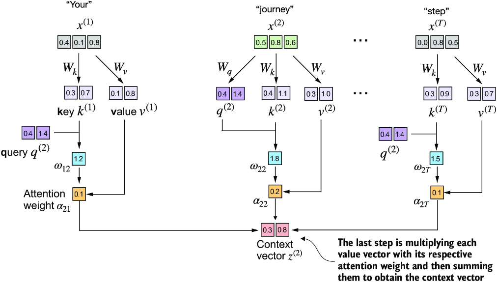
This attention mechanism was used in the original GPT implementation and is often referred to as scaled dot-product attention.
The main difference to the simplified self-attention mechanism is the introduction of three trainable weight matrices \(W_q\), \(W_k\), \(W_v\) (for query, key, and value respectively) that are used to project the embedded input tokens \(x^{(i)}\) into query, key, and value vectors respectively.
In the image below note that only the second token (“journey”) is projected into a query vector since only the second token is “being queried”. All T input tokens, however, are projected into key and value vectors (which will later be used to compute the full attention weight matrix).

A simple example (single query vector)
Unlike in the simplified self-attention mechanism, scaled dot-product attention computes attention scores not on raw token embeddings but on the tokens projected into key and value space (via weight matrices \(W_k\) and \(W_v\)).

Computing the normalized attention weights \(\alpha_{ij}\) from unnormalized attention scores \(\omega_{ij}\) is done via the softmax function as before. This time, however, we scale the attention scores by dividing them by the square root of the embedding dimension of the keys (hence the name scaled dot-product attention).
NOTE: The reason for the normalization by the embedding dimension size is to improve the training performance by avoiding small gradients. For instance, when scaling up the embedding dimension, which is typically greater than 1,000 for GPT-like LLMs, large dot products can result in very small gradients during backpropagation due to the softmax function applied to them. As dot products increase, the softmax function behaves more like a step function, resulting in gradients nearing zero. These small gradients can drastically slow down learning or cause training to stagnate (see page 69 in Sebastian Raschka’s book).

The last step is to compute the context vector for \(x^{(2)}\), which is the weighted sum of all value vectors of the input sequence (i.e. the input tokens embedded via the \(W_v\) matrix).
# Define input and output embedding size of the W_i embedding matrices.
# NOTE: For GPT-like models, the input embedding size is typically equal to the output embedding
#       size.
x_2 = inputs[1]  # Python uses 0-based indexing.
d_in = inputs.shape[1]  # The size of the input embedding dimension.
d_out = 2  # The size of the output embedding dimension.
print(f"Input token / shape: {x_2} ({x_2.shape})")

# Instantiate the trainable weight matrices.
# NOTE: requires_grad=False is done here to reduce visual clutter in the outputs. When training the
#       model, requires_grad obviously has to be set to True to update the weights during training.
torch.manual_seed(123)
W_q = torch.nn.Parameter(torch.randn(d_in, d_out), requires_grad=False)
W_k = torch.nn.Parameter(torch.randn(d_in, d_out), requires_grad=False)
W_v = torch.nn.Parameter(torch.randn(d_in, d_out), requires_grad=False)

# Project the query input token into query, key, and value vectors.
query_2 = x_2 @ W_q
key_2 = x_2 @ W_k
value_2 = x_2 @ W_v
print(f"Weight matrix shape: {W_q.shape}")
print(f"Projected query vector: {query_2}")

# Compute key and value vectors for all input tokens.
# NOTE: Computing the context vector for the query vector x(2) requires the key and value vectors of
#       all input tokens.
keys = inputs @ W_k
values = inputs @ W_v
print(f"Keys shape: {keys.shape}")
print(f"Values shape: {values.shape}")

# Compute the unnormalized attention scores (for the query vector x(2) first).
keys_2 = keys[1]
attn_scores_2 = query_2.dot(keys_2)
print(f"Unnormalized attention score for x^2: {attn_scores_2}")

# Compute the unnormalized attention scores for all input tokens.
attn_scores = query_2 @ keys.T
print(f"Unnormalized attention scores: {attn_scores}")

# Normalize the attention scores to get the attention weights.
d_k = keys.shape[1]
attn_weights = torch.nn.functional.softmax(attn_scores / d_k**0.5, dim=-1)
print(f"Attention weights: {attn_weights}")

# Compute the context vector for the query vector x(2).
context_vector_2 = torch.zeros(d_out)
for i, v_i in enumerate(values):
    context_vector_2 += attn_weights[i] * v_i

context_vector_2_mm = attn_weights @ values
assert torch.allclose(context_vector_2, context_vector_2_mm)
print(f"Context vector: {context_vector_2}")
Input token / shape: tensor([0.5500, 0.8700, 0.6600]) (torch.Size([3]))
Weight matrix shape: torch.Size([3, 2])
Projected query vector: tensor([-1.1729, -0.0048])
Keys shape: torch.Size([6, 2])
Values shape: torch.Size([6, 2])
Unnormalized attention score for x^2: 0.13763877749443054
Unnormalized attention scores: tensor([ 0.2172, 0.1376, 0.1730, -0.0491, 0.7616, -0.3809])
Attention weights: tensor([0.1704, 0.1611, 0.1652, 0.1412, 0.2505, 0.1117])
Context vector: tensor([0.2854, 0.4081])A self-attention class
In self-attention, we transform the input vectors in the input matrix X with the three weight matrices, \(W_q\), \(W_k\), and \(W_v\). The new compute the attention weight matrix based on the resulting queries (Q) and keys (K). Using the attention weights and values (V), we then compute the context vectors (Z).

class SelfAttentionV1(nn.Module):
    def __init__(self, d_in: int, d_out: int):
        super().__init__()
        self.W_q = nn.Parameter(torch.randn(d_in, d_out))
        self.W_k = nn.Parameter(torch.randn(d_in, d_out))
        self.W_v = nn.Parameter(torch.randn(d_in, d_out))

    def forward(self, x: torch.Tensor) -> torch.Tensor:
        # Project the input tokens into query, key, and value vectors.
        query = x @ self.W_q
        key = x @ self.W_k
        value = x @ self.W_v

        # Compute the unnormalized attention scores, i.e. the omegas.
        attn_scores = query @ key.T

        # Normalize the attention scores to get the attention weights, i.e. the alphas.
        d_k = key.shape[-1]
        attn_weights = torch.softmax(attn_scores / d_k**0.5, dim=-1)

        # Compute the full set of context vectors.
        context_vectors = attn_weights @ value

        return context_vectors


class SelfAttentionV2(nn.Module):
    """A Python class implementing self-attention.

    V2 replaces the nn.Parameter objects with nn.Linear objects which effectively perform matrix
    multiplication when the bias units are disabled.

    One significant advantage of using nn.Linear objects is that nn.Linear has an optimized weight
    initialization scheme that helps with stabilizing the training process and making it more
    effective.
    """

    def __init__(self, d_in: int, d_out: int, qkv_bias: bool = False):
        super().__init__()
        self.W_q = nn.Linear(d_in, d_out, bias=qkv_bias)
        self.W_k = nn.Linear(d_in, d_out, bias=qkv_bias)
        self.W_v = nn.Linear(d_in, d_out, bias=qkv_bias)

    def forward(self, x: torch.Tensor) -> torch.Tensor:
        # Project the input tokens into query, key, and value vectors.
        query = self.W_q(x)
        key = self.W_k(x)
        value = self.W_v(x)

        # Compute the unnormalized attention scores, i.e. the omegas.
        attn_scores = query @ key.T

        # Normalize the attention scores to get the attention weights, i.e. the alphas.
        d_k = key.shape[-1]
        attn_weights = torch.softmax(attn_scores / d_k**0.5, dim=-1)

        # Compute the full set of context vectors.
        context_vectors = attn_weights @ value

        return context_vectors


# Test the self-attention class.
torch.manual_seed(123)
sa_v1 = SelfAttentionV1(d_in, d_out)
sa_v2 = SelfAttentionV2(d_in, d_out)

# NOTE: SelfAttentionV1 and SelfAttentionV2 give different outputs because they use different
#       initial weights for the weight matrices since nn.Linear uses a more sophisticated weight
#       initialization scheme.
print(f"Context vector 2 (from before): {context_vector_2_mm}")
print(f"Context vectors (V1):\n{sa_v1(inputs)}")
print(f"Context vectors (V2):\n{sa_v2(inputs)}")
Context vector 2 (from before): tensor([0.2854, 0.4081])
Context vectors (V1):
tensor([[0.2845, 0.4071],
[0.2854, 0.4081],
[0.2854, 0.4075],
[0.2864, 0.3974],
[0.2863, 0.3910],
[0.2860, 0.4039]], grad_fn=<MmBackward0>)
Context vectors (V2):
tensor([[0.5322, 0.2491],
[0.5316, 0.2488],
[0.5316, 0.2488],
[0.5340, 0.2501],
[0.5331, 0.2497],
[0.5337, 0.2499]], grad_fn=<MmBackward0>)Causal self-attention
Causal attention or masked attention restricts a model to only consider previous and current inputs in a sequence when processing a given query token when computing attention scores (compare that to standard self-attention that considers the entire sequence as seen above).
Causal self-attention masks out future tokens such that the are not taken into account when computing context vectors. In the diagram below, any token above the diagonal of the attention matrix is a future token that should not be taken into account.
For example, the token “Your” can only attend to the first token in the sequence (i.e. “Your”) while the third token “starts” can attend to all prior tokens as well, i.e. “Your”, “journey”, and “starts”.

The causal self-attention implementation will modify our previous self-attention implementation by introducing a mask to modify the attention weight matrix.

The above implementation results in wasted computation since we still compute the full attention matrix and normalize twice (once in the softmax operation on the full attention matrix and once after masking out upper triangular entries). A more efficient implementation below relies on a property of the softmax function (where negative infinity entries in the attention matrix are essentially zero probability entries). Mathematically, this occurs because \(e^{-\infty} \rightarrow 0\).

# Compute the attention scores.
# NOTE: Reuses the query and key weight matrices of the SelfAttention_v2 object from the previous
#       section for convenience
queries = sa_v2.W_q(inputs)
keys = sa_v2.W_k(inputs)
attn_scores = queries @ keys.T
attn_weights = torch.softmax(attn_scores / keys.shape[-1] ** 0.5, dim=-1)
print(f"Attention weights:\n{attn_weights}")

# Simple mask with 0s above the main diagonal
# NOTE: torch.tril creates a lower triangular matrix with ones on and below the diagonal.
context_length = attn_scores.shape[0]
mask_simple = torch.tril(torch.ones(context_length, context_length)).type(torch.int64)
print(f"\nSimple mask:\n{mask_simple}")

# Create a mask with negative infinity entries for the upper triangular entries.
# NOTE: torch.triu creates an upper triangular matrix with ones on and above the diagonal.
context_length = attn_weights.shape[0]
mask = torch.triu(torch.ones(context_length, context_length), diagonal=1).type(
    torch.int64
)
print(f"\nMask (for softmax):\n{mask}")

# Apply the mask to the attention scores.
attn_weights_masked = attn_weights.masked_fill(mask.bool(), -torch.inf)
print(f"\nAttention weights masked:\n{attn_weights_masked}")

# Normalize the masked attention weights.
attn_weights_masked_normalized = torch.softmax(
    attn_weights_masked / keys.shape[-1] ** 0.5, dim=1
)
print(f"\nAttention weights masked and normalized:\n{attn_weights_masked_normalized}")
Attention weights:
tensor([[0.1825, 0.1568, 0.1576, 0.1657, 0.1796, 0.1577],
[0.1852, 0.1554, 0.1562, 0.1655, 0.1814, 0.1563],
[0.1852, 0.1554, 0.1562, 0.1654, 0.1814, 0.1563],
[0.1756, 0.1611, 0.1615, 0.1662, 0.1740, 0.1616],
[0.1804, 0.1589, 0.1594, 0.1655, 0.1765, 0.1593],
[0.1760, 0.1605, 0.1610, 0.1664, 0.1749, 0.1612]],
grad_fn=<SoftmaxBackward0>)
Simple mask:
tensor([[1, 0, 0, 0, 0, 0],
[1, 1, 0, 0, 0, 0],
[1, 1, 1, 0, 0, 0],
[1, 1, 1, 1, 0, 0],
[1, 1, 1, 1, 1, 0],
[1, 1, 1, 1, 1, 1]])
Mask (for softmax):
tensor([[0, 1, 1, 1, 1, 1],
[0, 0, 1, 1, 1, 1],
[0, 0, 0, 1, 1, 1],
[0, 0, 0, 0, 1, 1],
[0, 0, 0, 0, 0, 1],
[0, 0, 0, 0, 0, 0]])
Attention weights masked:
tensor([[0.1825, -inf, -inf, -inf, -inf, -inf],
[0.1852, 0.1554, -inf, -inf, -inf, -inf],
[0.1852, 0.1554, 0.1562, -inf, -inf, -inf],
[0.1756, 0.1611, 0.1615, 0.1662, -inf, -inf],
[0.1804, 0.1589, 0.1594, 0.1655, 0.1765, -inf],
[0.1760, 0.1605, 0.1610, 0.1664, 0.1749, 0.1612]],
grad_fn=<MaskedFillBackward0>)
Attention weights masked and normalized:
tensor([[1.0000, 0.0000, 0.0000, 0.0000, 0.0000, 0.0000],
[0.5053, 0.4947, 0.0000, 0.0000, 0.0000, 0.0000],
[0.3380, 0.3309, 0.3311, 0.0000, 0.0000, 0.0000],
[0.2517, 0.2491, 0.2492, 0.2500, 0.0000, 0.0000],
[0.2017, 0.1987, 0.1988, 0.1996, 0.2012, 0.0000],
[0.1678, 0.1659, 0.1660, 0.1666, 0.1676, 0.1660]],
grad_fn=<SoftmaxBackward0>)Dropout: Masking additional attention weights
Dropout is a technique where randomly selected hidden layer units are ignored (or dropped out) which helps prevent overfitting during training because the model is not allowed to become overly reliant on any specific set of hidden layer units. Note that dropout is only used during training and disabled afterwards.
Dropout in self-attention is most commonly applied at two specific times: 1. after calculating the attention weights 2. after applying the attention weights to the value vectors
Here we’ll apply dropout after applying the attention weights to the value vectors (which is the more common variant in practice).

torch.manual_seed(123)
# Instantiate the dropout module (choose a dropout probability of 50%)
dropout = torch.nn.Dropout(p=0.5)

# Create some example data (a matrix of ones).
example = torch.ones(6, 6)
print(f"Example:\n{example}")

# NOTE: Applying dropout scales the outputs by a factor of 1/(1-p) during training. This means that
#       during evaluation the module simply computes an identity function. This is done to compensate
#       for the reduction of active elements and is crucial to maintain the overall balance of the
#       attention weights as it ensures that the average influence of the attention mechanism remains
#       consistent during both the training and inference phases.
# See https://pytorch.org/docs/stable/generated/torch.nn.Dropout.html
print(f"Dropout:\n{dropout(example)}")

# Apply dropout to the attention weights.
print(f"Dropout:\n{dropout(attn_weights_masked_normalized)}")
Example:
tensor([[1., 1., 1., 1., 1., 1.],
[1., 1., 1., 1., 1., 1.],
[1., 1., 1., 1., 1., 1.],
[1., 1., 1., 1., 1., 1.],
[1., 1., 1., 1., 1., 1.],
[1., 1., 1., 1., 1., 1.]])
Dropout:
tensor([[2., 2., 2., 2., 2., 2.],
[0., 2., 0., 0., 0., 0.],
[0., 0., 2., 0., 2., 0.],
[2., 2., 0., 0., 0., 2.],
[2., 0., 0., 0., 0., 2.],
[0., 2., 0., 0., 0., 0.]])
Dropout:
tensor([[2.0000, 0.0000, 0.0000, 0.0000, 0.0000, 0.0000],
[0.0000, 0.0000, 0.0000, 0.0000, 0.0000, 0.0000],
[0.0000, 0.0000, 0.6622, 0.0000, 0.0000, 0.0000],
[0.0000, 0.4982, 0.0000, 0.5000, 0.0000, 0.0000],
[0.0000, 0.3974, 0.3975, 0.3993, 0.4024, 0.0000],
[0.3355, 0.3319, 0.0000, 0.0000, 0.3353, 0.3320]],
grad_fn=<MulBackward0>)A compact causal attention class
# We want to ensure that our implementation works with batches of data (as produced by the
# dataloader implemented in chapter 2).
batch = torch.stack([inputs, inputs], dim=0)
print(f"Batch shape: {batch.shape}")


class CausalAttention(nn.Module):
    def __init__(
        self,
        d_in: int,
        d_out: int,
        context_length: int,
        dropout_prob: float = 0.1,
        qkv_bias: bool = False,
    ):
        super().__init__()
        # Cache d_out for later use.
        self.d_out = d_out

        # Initialize the weight matrices.
        self.W_q = nn.Linear(d_in, d_out, bias=qkv_bias)
        self.W_k = nn.Linear(d_in, d_out, bias=qkv_bias)
        self.W_v = nn.Linear(d_in, d_out, bias=qkv_bias)

        # Initialize the dropout module.
        # Compared to the previous implementation, we now use a dropout layer.
        self.dropout = torch.nn.Dropout(p=dropout_prob)

        # Register a buffer for the mask.
        # NOTE: Buffers are not trained and are not subject to gradient descent.
        # NOTE: The use of register_buffer in PyTorch is not strictly necessary for all use cases
        #       but offers several advantages here. For instance, when we use the CausalAttention
        #       class in our LLM, buffers are automatically moved to the appropriate device (CPU or
        #       GPU) along with our model, which will be relevant when training our LLM. This means
        #       we don’t need to manually ensure these tensors are on the same device as your model
        #       parameters, avoiding device mismatch errors.
        self.register_buffer(
            "mask", torch.triu(torch.ones(context_length, context_length), diagonal=1)
        )

    def forward(self, x: torch.Tensor, verbose: bool = False) -> torch.Tensor:
        # Extract input dimensions.
        batch_size, num_tokens, d_in = x.shape

        # Project input into query, key, and value vectors.
        query = self.W_q(x)
        key = self.W_k(x)
        value = self.W_v(x)

        # Compute the unnormalized attention scores.
        # NOTE: We transpose dimensions 1 and 2, keeping the batch dimension at the first position (0).
        attn_scores = query @ key.transpose(-2, -1)

        # Apply the mask to the attention scores.
        # NOTE: In PyTorch, operations with a trailing underscore are performed in-place, avoiding
        #       unnecessary memory copies.
        attn_scores.masked_fill_(self.mask.bool()[:num_tokens, :num_tokens], -torch.inf)
        if verbose:
            print(
                f"Unnormalized causal attention scores (shape: {attn_scores.shape}):\n{attn_scores}"
            )

        # Normalize the attention scores.
        attn_weights = torch.softmax(attn_scores / self.d_out**0.5, dim=-1)
        if verbose:
            print(
                f"Normalized causal attention weights (shape: {attn_weights.shape}):\n{attn_weights}"
            )

        # Apply dropout to the attention weights.
        attn_weights = self.dropout(attn_weights)

        # Compute the context vectors.
        context_vectors = attn_weights @ value
        if verbose:
            print(
                f"Context vectors (shape: {context_vectors.shape}):\n{context_vectors}"
            )

        return context_vectors


# Test the causal attention class.
torch.manual_seed(123)
context_length = batch.shape[1]
ca = CausalAttention(d_in, d_out, context_length, 0.0)
context_vecs = ca(batch)
print(f"Context vector shape: {context_vecs.shape}")
Batch shape: torch.Size([2, 6, 3])
Context vector shape: torch.Size([2, 6, 2])Multi-head self-attention (naive)
The term “multi-head” refers to dividing the attention mechanism into multiple “heads,” each operating independently. In this context, a single causal attention module can be considered single-head attention, where there is only one set of attention weights processing the input sequentially.
In a basic implementation of multi-head self-attention, one could just stack multiple causal self-attention modules as is done in the following figure and the MultiHeadAttentionWrapper below. Each head has its own weights and all heads’ outputs are combined by stacking the output tensors. This is a rather inefficient implementation since the individual heads are processed sequentially.
Using multiple instances of the self-attention mechanism can be computationally intensive, but it’s crucial for the kind of complex pattern recognition that models like transformer-based LLMs are known for.
As mentioned before, the main idea behind multi-head attention is to run the attention mechanism multiple times (in parallel) with different, learned linear projections—the results of multiplying the input data (like the query, key, and value vectors in attention mechanisms) by a weight matrix.

The example below shows how the individual heads compute their output and how the output tensors are stacked.

class MultiHeadAttentionWrapper(nn.Module):
    def __init__(
        self,
        d_in: int,
        d_out: int,
        context_length: int,
        dropout: float,
        num_heads: int,
        qkv_bias: bool = False,
    ):
        """Initialize the multi-head attention wrapper.

        Args:
            d_in: The dimension of the input.
            d_out: The dimension of the output.
            context_length: The length of the context. This argument sets the length of the causal
                mask, i.e. the maximum supported sequence length.
            dropout: The dropout probability.
            num_heads: The number of attention heads.
            qkv_bias: Whether to use a bias in the query, key, and value projections.
        """
        super().__init__()
        self.heads = nn.ModuleList(
            [
                CausalAttention(d_in, d_out, context_length, dropout, qkv_bias)
                for _ in range(num_heads)
            ]
        )

    def forward(self, x):
        # NOTE: All heads are processed sequentially which is inefficient.
        return torch.cat([head(x) for head in self.heads], dim=-1)


# Test with a simple example.
torch.manual_seed(123)
context_length = batch.shape[1]  # This is the number of tokens
d_in, d_out = 3, 2

mha = MultiHeadAttentionWrapper(
    d_in=d_in, d_out=d_out, context_length=context_length, dropout=0.0, num_heads=2
)
context_vecs = mha(batch)

# NOTE: The shapes below indicate that the input batch (shape [2,6,3]) is transformed into a tensor
#       of shape [2,6,4] where the last dimension is the concatenation of the outputs of the two heads.
# Input size:                       [2,6,3] (last dim is d_in)
# Individual head output size:      [2,6,2] (last dim is d_out)
# Concatenated head output size:    [2,6,4] (last dim is d_out * num_heads)
print(f"Context vectors:\n{context_vecs}")
print(f"Batch shape: {batch.shape}")
print(f"Context vectors shape: {context_vecs.shape}")
Context vectors:
tensor([[[-0.4519, 0.2216, 0.4772, 0.1063],
[-0.5874, 0.0058, 0.5891, 0.3257],
[-0.6300, -0.0632, 0.6202, 0.3860],
[-0.5675, -0.0843, 0.5478, 0.3589],
[-0.5526, -0.0981, 0.5321, 0.3428],
[-0.5299, -0.1081, 0.5077, 0.3493]],
[[-0.4519, 0.2216, 0.4772, 0.1063],
[-0.5874, 0.0058, 0.5891, 0.3257],
[-0.6300, -0.0632, 0.6202, 0.3860],
[-0.5675, -0.0843, 0.5478, 0.3589],
[-0.5526, -0.0981, 0.5321, 0.3428],
[-0.5299, -0.1081, 0.5077, 0.3493]]], grad_fn=<CatBackward0>)
Batch shape: torch.Size([2, 6, 3])
Context vectors shape: torch.Size([2, 6, 4])Multi-head self-attention (parallel)
One way to improve the efficiency of multi-head self-attention (MHA) is by computing the outputs for all attention heads simultaneously via matrix multiplication.
The CausalAttention class independently performs the attention mechanism, and the results from each head are concatenated. In contrast, the following MultiHeadAttention class integrates the multi-head functionality within a single class. It splits the input into multiple heads by reshaping the projected query, key, and value tensors and then combines the results from these heads after computing attention.
The below image compares the two implementations. In the MultiHeadAttentionWrapper class with two attention heads, we initialized two weight matrices, \(W_{q_1}\) and \(W_{q_2}\), and computed two query matrices, \(Q_1\) and \(Q_2\) (top). In the MultiheadAttention class, we initialize one larger weight matrix \(W_q\), only perform one matrix multiplication with the inputs to obtain a query matrix Q, and then split the query matrix into \(Q_1\) and \(Q_2\) (bottom).
The splitting of the query, key, and value tensors is achieved through tensor reshaping and transposing operations using PyTorch’s .view and .transpose methods. The input is first transformed (via linear layers for queries, keys, and values) and then reshaped to represent multiple heads.

class MultiHeadAttention(nn.Module):
    def __init__(
        self,
        d_in: int,
        d_out: int,
        context_length: int,
        dropout: float,
        num_heads: int,
        qkv_bias: bool = False,
    ):
        """Initialize the multi-head attention class.

        Args:
            d_in: The dimension of the input.
            d_out: The dimension of the output.
            context_length: The length of the context. This argument sets the length of the causal
                mask, i.e. the maximum supported sequence length.
            dropout: The dropout probability.
            num_heads: The number of attention heads.
            qkv_bias: Whether to use a bias in the query, key, and value projections.
        """
        super().__init__()

        # Verify that the output dimension is divisible by the number of heads, which is required
        # for splitting the output into the specified number of heads.
        assert d_out % num_heads == 0, "d_out must be divisible by num_heads"

        # Cache the output dimension and the number of heads for later use.
        # NOTE: This reduces the projection dim to match the desired output dim.
        # NOTE: The key operation is to split the d_out dimension into num_heads and head_dim,
        #       where head_dim = d_out / num_heads. This splitting is then achieved using the .view
        #       method: a tensor of dimensions (b, num_tokens, d_out) is reshaped to dimension
        #       (b, num_tokens, num_heads, head_dim).
        self.d_out = d_out
        self.num_heads = num_heads
        self.head_dim = d_out // num_heads

        # Initialize the weight matrices.
        # NOTE: Only a single weight matrix is initialized for the query, key, and value projections
        #       since we will split the output into the specified number of heads.
        self.W_q = nn.Linear(d_in, d_out, bias=qkv_bias)
        self.W_k = nn.Linear(d_in, d_out, bias=qkv_bias)
        self.W_v = nn.Linear(d_in, d_out, bias=qkv_bias)

        # Initialize the output projection layer.
        # NOTE: This implementation uses a Linear layer to combine all head outputs.
        self.out_proj = nn.Linear(d_out, d_out)

        # Initialize the dropout layer.
        self.dropout = nn.Dropout(dropout)

        # Register a buffer for the mask.
        self.register_buffer(
            "mask", torch.triu(torch.ones(context_length, context_length), diagonal=1)
        )

    def forward(self, x: torch.Tensor) -> torch.Tensor:
        # Extract input dimensions.
        # NOTE: The customary notation for these dimensions is [B, T, D] where:
        #
        #   B = batch size
        #   T = sequence length (num_tokens)
        #   D = model dimension (d_in)
        b, num_tokens, d_in = x.shape

        # Project the input into query, key, and value vectors.
        # NOTE: The shape of the projected query, key, and value vectors is [B, T, D]
        keys = self.W_k(x)  # [B, T, D]
        queries = self.W_q(x)  # [B, T, D]
        values = self.W_v(x)  # [B, T, D]
        print(f"keys.shape: {keys.shape}")
        print(f"queries.shape: {queries.shape}")
        print(f"values.shape: {values.shape}")

        # Split the query, key, and value vectors into the specified number of heads.
        # NOTE: We implicitly split the matrix by adding a num_heads dimension. Then we unroll the
        #       last dim: (b, num_tokens, d_out) -> (b, num_tokens, num_heads, head_dim).
        # Compute head dimension
        head_dim = self.d_out // self.num_heads
        print(f"head_dim: {head_dim}")

        # Reshape to [B, T, H, D_h] where:
        #
        #   B = batch size
        #   T = sequence length (num_tokens)
        #   H = number of heads
        #   D_h = dimension per head (head_dim)
        #
        # NOTE: We implicitly split the matrix by adding a num_heads dimension. Then we unroll the
        #       last dim: (b, num_tokens, d_out) -> (b, num_tokens, num_heads, head_dim).
        # NOTE: See section "A note on views" for more details.
        keys = keys.view(b, num_tokens, self.num_heads, head_dim)
        values = values.view(b, num_tokens, self.num_heads, head_dim)
        queries = queries.view(b, num_tokens, self.num_heads, head_dim)
        print(f"keys.shape: {keys.shape}")
        print(f"values.shape: {values.shape}")
        print(f"queries.shape: {queries.shape}")

        # Transpose from [B, T, H, D_h] to [B, H, T, D_h], i.e. from shape
        # (b, num_tokens, num_heads, head_dim) to (b, num_heads, num_tokens, head_dim)
        #
        # NOTE: This transposition is crucial for correctly aligning the queries, keys, and values
        #       across the different heads and performing batched matrix multiplications
        #       efficiently.
        # NOTE: This reshaping results in each head having access to the full sequence of tokens
        #       (i.e. a tensor of shape T x D_h).
        keys = keys.transpose(1, 2)  # shape [B, H, T, D_h]
        queries = queries.transpose(1, 2)  # shape [B, H, T, D_h]
        values = values.transpose(1, 2)  # shape [B, H, T, D_h]
        print(f"keys.shape: {keys.shape}")
        print(f"values.shape: {values.shape}")
        print(f"queries.shape: {queries.shape}")

        # Compute the unnormalized attention scores via a dot product for each head.
        # NOTE: We transpose the T and D_h dimension (i.e. num_tokens and head_dim) just like we
        #       have already done in the "Trainable self-attention" section.
        # NOTE: Change key shape from [B, H, T, D_h] to [B, H, D_h, T]
        # NOTE: The output shape of attn_scores is [B, H, T, T], i.e. a square matrix of size T
        #       (i.e. sequence length) for each head.
        # NOTE: The following operation does a batched matrix multiplication between queries and
        #       keys. In this case, the matrix multiplication implementation in PyTorch handles the
        #       four-dimensional input tensor so that the matrix multiplication is carried out
        #       between the two last dimensions (num_tokens, head_dim) and then repeated for the
        #       individual heads.
        # NOTE: See section "A note on batched matrix multiplications" for more details.
        attn_scores = queries @ keys.transpose(2, 3)  # shape [B, H, T, T]
        print(f"attn_scores.shape: {attn_scores.shape}")

        # The mask is truncated to the number of tokens in the input sequence (i.e. sequence
        # length T)
        mask_bool = self.mask.bool()[:num_tokens, :num_tokens]  # shape [T, T]
        print(f"mask_bool.shape: {mask_bool.shape}")

        # Apply the mask to the attention scores.
        attn_scores.masked_fill_(mask_bool, -torch.inf)  # shape [B, H, T, T]

        # Compute the normalized attention weights (as before)
        # NOTE: The scaling factor is the last dimension of the keys tensor (i.e. head_dim, see
        #       line 88).
        attn_weights = torch.softmax(attn_scores / keys.shape[-1] ** 0.5, dim=-1)
        attn_weights = self.dropout(attn_weights)  # shape [B, H, T, T]
        print(f"attn_weights.shape: {attn_weights.shape}")

        # Compute the context vectors.
        # NOTE: The shapes of the individual tensors are:
        #       - attn_weights: [B, H, T, T]
        #       - values: [B, H, T, D_h]
        #       - context_vec: [B, H, T, D_h]
        #       - context_vec.transposed: [B, T, H, D_h]
        # NOTE: The context vectors from all heads are transposed back to the shape
        #       (b, num_tokens, num_heads, head_dim).
        context_vec = (attn_weights @ values).transpose(1, 2)  # shape [B, T, H, D_h]
        print(f"context_vec.shape: {context_vec.shape}")

        # Reshape/flatten the context vectors from [B, T, H, D_h] to [B, T, D_out], i.e. combine all
        # individual attention heads (d_out = H * D_h).
        # NOTE: Combines heads, where self.d_out = self.num_heads * self.head_dim (see line 32).
        context_vec = context_vec.contiguous().view(b, num_tokens, self.d_out)
        print(f"context_vec.shape: {context_vec.shape}")

        # Optionally project the context vectors to the output dimension.
        # NOTE: This output projection layer is not strictly necessary (see appendix B of the book
        #       for more details), but it is commonly used in many LLM architectures.
        context_vec = self.out_proj(context_vec)
        return context_vec


# Test with a simple example.
torch.manual_seed(123)
batch_size, context_length, d_in = batch.shape
d_out = 2
mha = MultiHeadAttention(d_in, d_out, context_length, 0.0, num_heads=2)
context_vecs = mha(batch)
print(context_vecs)
print("context_vecs.shape:", context_vecs.shape)
keys.shape: torch.Size([2, 6, 2])
queries.shape: torch.Size([2, 6, 2])
values.shape: torch.Size([2, 6, 2])
head_dim: 1
keys.shape: torch.Size([2, 6, 2, 1])
values.shape: torch.Size([2, 6, 2, 1])
queries.shape: torch.Size([2, 6, 2, 1])
keys.shape: torch.Size([2, 2, 6, 1])
values.shape: torch.Size([2, 2, 6, 1])
queries.shape: torch.Size([2, 2, 6, 1])
attn_scores.shape: torch.Size([2, 2, 6, 6])
mask_bool.shape: torch.Size([6, 6])
attn_weights.shape: torch.Size([2, 2, 6, 6])
context_vec.shape: torch.Size([2, 6, 2, 1])
context_vec.shape: torch.Size([2, 6, 2])
tensor([[[0.3190, 0.4858],
[0.2943, 0.3897],
[0.2856, 0.3593],
[0.2693, 0.3873],
[0.2639, 0.3928],
[0.2575, 0.4028]],
[[0.3190, 0.4858],
[0.2943, 0.3897],
[0.2856, 0.3593],
[0.2693, 0.3873],
[0.2639, 0.3928],
[0.2575, 0.4028]]], grad_fn=<ViewBackward0>)
context_vecs.shape: torch.Size([2, 6, 2])A note on views
# Example for reshaping a tensor from [2, 3, 4] to [2, 3, 2, 2] (via views)
B, T, D = 2, 3, 4
x = torch.randn((B, T, D))
print(x.shape)
x_view = x.view(B, T, 2, 2)
print(x_view.shape)
torch.Size([2, 3, 4])
torch.Size([2, 3, 2, 2])A note on batched matrix multiplications
# The shape of this tensor is (b, num_heads, num_tokens, head_dim) = (1, 2, 3, 4).
a = torch.tensor(
    [
        [
            [
                [0.2745, 0.6584, 0.2775, 0.8573],
                [0.8993, 0.0390, 0.9268, 0.7388],
                [0.7179, 0.7058, 0.9156, 0.4340],
            ],
            [
                [0.0772, 0.3565, 0.1479, 0.5331],
                [0.4066, 0.2318, 0.4545, 0.9737],
                [0.4606, 0.5159, 0.4220, 0.5786],
            ],
        ]
    ]
)

# Perform a batched matrix multiplication between a and a.transpose(2, 3), i.e. num_tokens and
# head_dim are transposed.
# NOTE: [1, 2, 3, 4] @ [1, 2, 4, 3] = [1, 2, 3, 3]
# NOTE: In this case, the matrix multiplication implementation in PyTorch handles the
#       four-dimensional input tensor so that the matrix multiplication is carried out between the
#       two last dimensions (num_tokens, head_dim) and then repeated for the individual heads (as
#       well as for each batch separately, i.e. the first dimension which here is just one element).
aat = a @ a.transpose(2, 3)
print(f"Shape of aat: {aat.shape}")
print(aat)
Shape of aat: torch.Size([1, 2, 3, 3])
tensor([[[[1.3208, 1.1631, 1.2879],
[1.1631, 2.2150, 1.8424],
[1.2879, 1.8424, 2.0402]],
[[0.4391, 0.7003, 0.5903],
[0.7003, 1.3737, 1.0620],
[0.5903, 1.0620, 0.9912]]]])# A less compact version of the above operation is as follows:
first_head = a[0, 0, :, :]
first_res = first_head @ first_head.T
print("First head:\n", first_res)
second_head = a[0, 1, :, :]
second_res = second_head @ second_head.T
print("\nSecond head:\n", second_res)First head:
tensor([[1.3208, 1.1631, 1.2879],
[1.1631, 2.2150, 1.8424],
[1.2879, 1.8424, 2.0402]])
Second head:
tensor([[0.4391, 0.7003, 0.5903],
[0.7003, 1.3737, 1.0620],
[0.5903, 1.0620, 0.9912]])